Correlation coefficients through online marketing examples

Reading Time: 12 minutes

Through this post we will introduce you to the simple mathematical concept – the theory of correlation coefficients. The interpretation and application of this theory allow us to analyze the relationship between variables. We will explain, in detail, some ideas that lie behind the theory.

If you don’t understand all the concepts, don’t panic. For those not interested in mathematics, it is enough to gain intuition by understanding the interpretation of correlation coefficients that we will present. We are exploring the theory of correlation coefficients through examples in online advertising

Correlation analysis is the most basic way of mathematically connecting the dots between variables. We use this statistical method to evaluate the strength of the relationship between two quantitative variables.

Although scatter plots provide a lot of visual information, it can be helpful to assess the relationship between points. One measure of the relationship between two variables is the covariance.

More about covariance

Covariance is a measure of the joint variability of two random variables. It can be defined if the second moments of the analyzed variables are finite. The mathematical definition is as follows:

Basic mathematical definition of covariance

Therefore, covariance is the arithmetic mean of the products of the deviation of the value of the variable x from its arithmetic mean, and the value of the variable y from its arithmetic mean. As a descriptive statistical measure, we can calculate it by the following formula:

Derived covariance formula (for asymptotically normally distributed variables)

To illustrate, if values x and y tend to go in the same direction across observations, either higher or lower than their respective means, then they have a positive covariance. If the covariance is zero, then there is no association between x and y. A negative covariance means that the variables go in opposite directions relative to their means: when x is lower, y is higher.

The following plot is a graphical representation of variables over time with different covariance values. We see the relationship of total SPEND, CR (Conversion Rate), and CAC (Customer Acquisition Cost) with the total number of PURCHASES. The first graph shows an example of positive covariance (3273.761) between purchases and spend over time.

The second graph shows the negative covariance between CAC and purchases (covariance is -46,872). In the last graph, we see an example of a connection whose covariance is about 0.

Three images showing different covariance values. (Positive covariance, negative covariance and covariance is approximately 0).

About correlation: the strength of association

Formally, correlation represents the connections between statistical variables which tend to vary, are associated, or occur together in a way not expected by chance. We can expressed the significance and strength of these connections by various measures.

A high correlation means that variables have a strong relationship with each other, while a weak correlation means that the variables are hardly related. 

The most important fact is that correlation does not imply causation. In other words, seeing two variables moving together does not necessarily mean we know whether one variable change causes the other to occur. 

In statistics, a spurious correlation refers to a connection between two variables that appears causal but is not. At this link, you can see interesting examples of this term (possible misinterpretations of correlations).

In this post, we will only consider the correlations of two variables, also called a bivariate correlation. If the variables are continuous, we can show them on a scatter plot. The figure below shows the values of CAC and CR over time.

The first image shows the scaled original points, and the second shows them after geometrical smoothing. It is clear from the figure that CAC and CR increase and decrease together, therefore, they are highly correlated. But how would you rate the strength of the connection from -1 to 1? We will answer this question later.

two plot

The correlation coefficient shows the true strength of the correlation

A correlation coefficient is a numerical measure of some type of correlation, meaning a statistical relationship between two variables. When we draw a conclusion, we often use words such as perfect, strong, good, or weak to describe the strength of the relationship between variables.

The same strength of the correlation coefficient is named differently by several researchers. The most popular method to perform correlation analysis is the Pearson correlation coefficient, but it is not always a good choice. When we do not meet the assumptions, we use non-parametric ranking tests, such as Kendall’s tau and Spearman’s rho.

Pearson correlation coefficient

It is difficult to interpret the size of covariance because the scale depends on the variables involved. The covariance will be different if the variables are measured in different units of measurement.

Hence, it is helpful to scale the covariance by the standard deviation for each variable, which results in a standardized, rescaled correlation coefficient known as the Pearson product-moment correlation coefficient, often marked as the symbol r:

Basic definition of the Pearson correlation coefficient. Covariance through the product of standard deviations.

It’s also known as a parametric correlation test because it depends on data distribution. We can use it only when x and y are from a normal distribution, without outliers.

This technique is strictly connected to the linear regression analysis which is a statistical approach for modeling the association between dependent and independent variables. As a result, we can plot a linear regression curve. See a more detailed explanation of how brand awareness is influenced by acquisition campaigns in our blog post.

Simple interpretation of the Pearson correlation coefficient

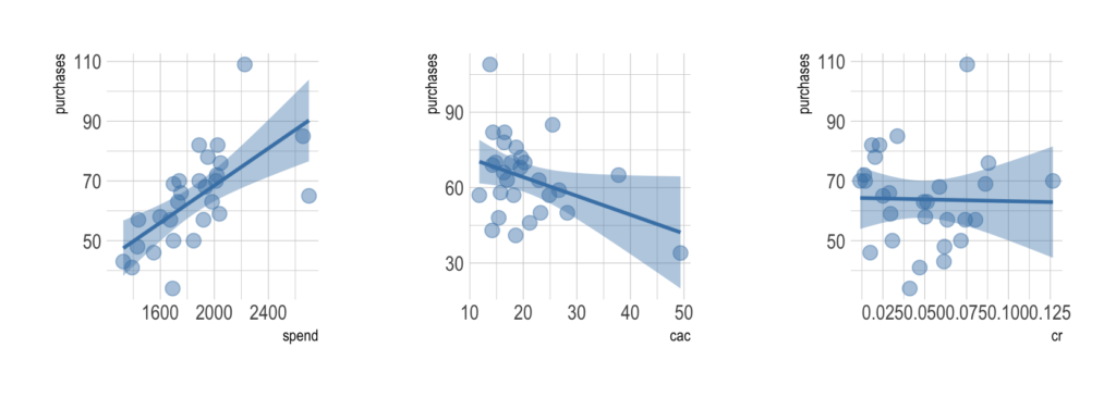
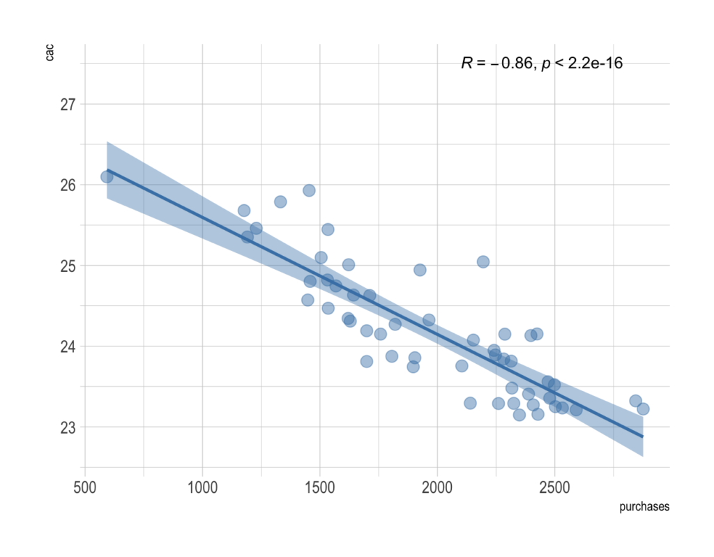
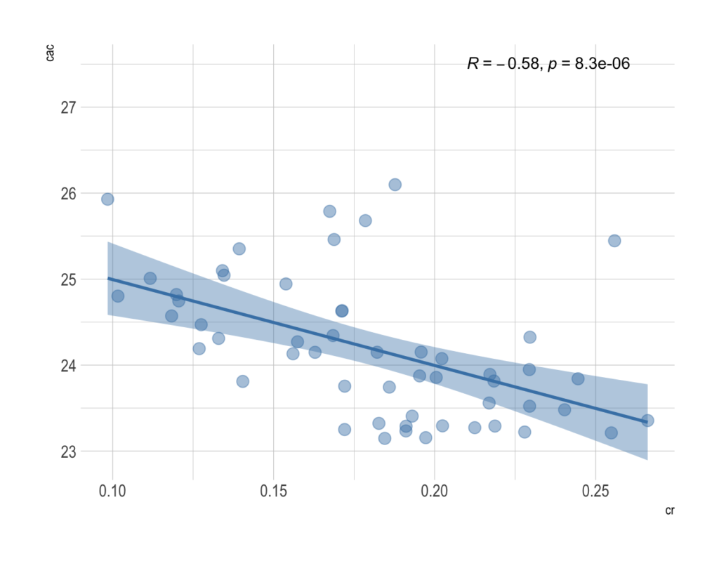
Pearson’s r is a continuous metric that falls in the range [-1, 1]. It is 1 in the case of a perfect positive linear association between the two variables, and -1 for a perfect negative linear association. If there is little or no linear association, r will be near 0. A negative r means that the variables are inversely related.

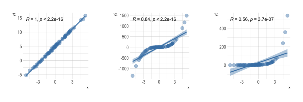
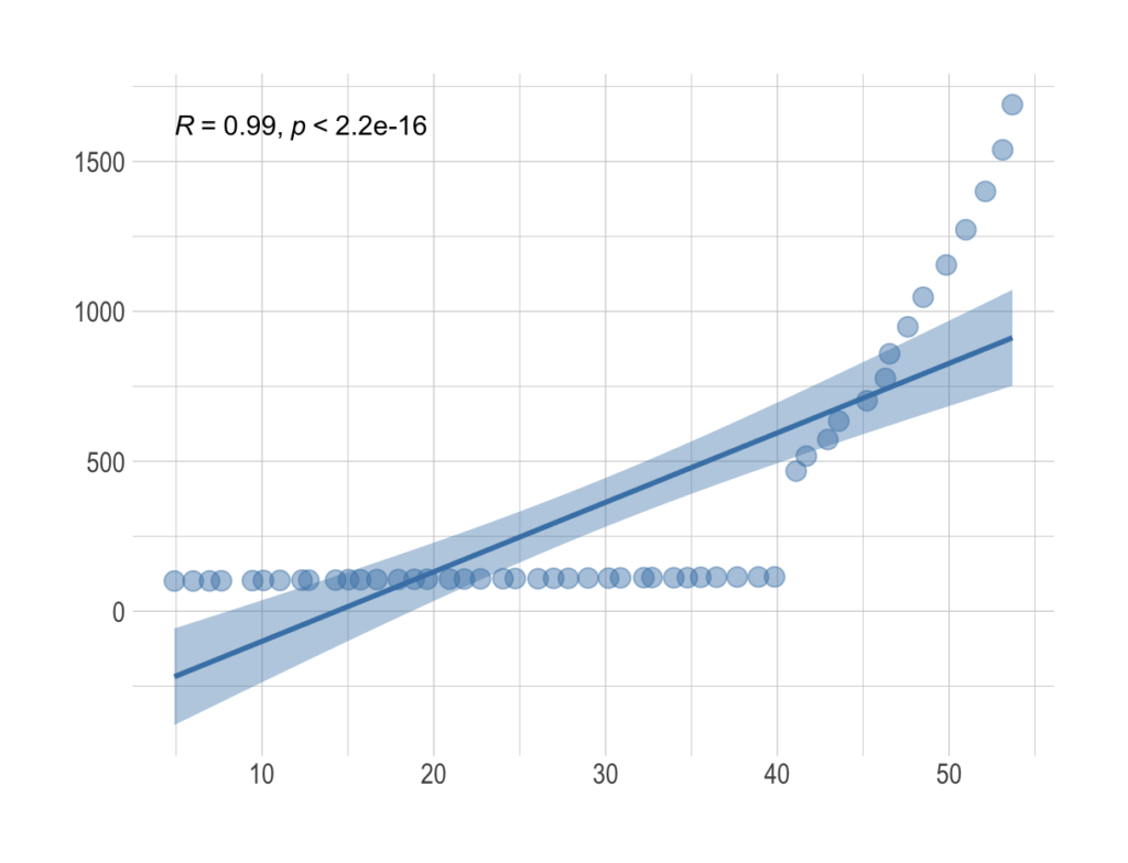
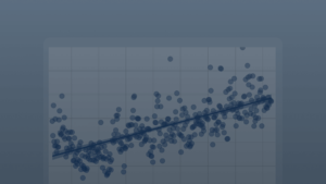
On a scatter plot, data with perfect association would have all points along a straight line. This makes r an easily interpreted metric to assess whether two variables have a close linear association or not.

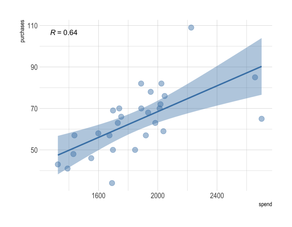
By squaring the value of the coefficient, we get the coefficient of determination, which we denote by . It determines how much variation of the data is explained by the linear model. 

Example 1

We observe the relationship between spend and purchases for a certain time, shown in the following graph.

Example with a medium-strong significant Pearson correlation coefficient.

The variables are normally distributed so we can use Pearson’s r to explore relationships. The value of the coefficient is 0.64  which indicates a positive relationship (we could say it is moderate). The graph also shows a fit regression curve, along with reliable intervals.

This linear model explains 41% of the variation in the data. Because some outliers are visible so it might be better to use some other correlation coefficient.

What is the idea behind the rank correlation coefficients?

In general, ranking tests have a very simple idea. Each variable is ranked separately from lowest to highest. So, a rank correlation coefficient measures the degree of similarity between two rankings. An increasing rank correlation coefficient implies an increasing agreement between rankings. The coefficient is inside the interval [-1, 1], and assumes the value:

  • 1 if the agreement between the two rankings is perfect (the two rankings are the same).
  • 0 if the rankings are completely independent.
  • -1 if the disagreement between the two rankings is perfect (one ranking is the reverse of the other).

Additionally, when we have two same values in the data (called a “tie”), we need to take the average of the ranks that they would have otherwise occupied. See more here.

We will describe the two most well-known rank correlation coefficients already mentioned. 

Spearman rank correlation coefficient

Spearman’s rank correlation coefficient  (rho) is a nonparametric (distribution-free) rank statistic proposed as a measure of the strength of the association between two variables. It is a measure of monotone association used when the distribution of data makes Pearson’s r undesirable or misleading. Intuitively, if we have a set of n pairs , we replace the data pairs with their ranks, and compute Pearson’s correlation coefficient based on the ranks.

This assesses how well an arbitrary monotonic function can describe the relationship between two variables, without making any assumptions about the distributions. So, rs shows if there is a monotone relationship between two variables and we can interpret it as follows:

  • – There is no monotonic connection
  • – There is a growing connection
  • – There is a falling connection

This coefficient is used when at least one variable is ordinal. We calculate it using derived expressions:

derived expressions

where  is rank difference. For a detailed derivation of the formula, see the following link. If the data is correlated, then the sum of squares of the difference between ranks will be small. Depending on the amount, the correlation may or may not be significant.

Kendall’s tau

Tau () is another nonparametric rank correlation coefficient that is used to understand the strength of the relationship between two variables. It is in the same range as other correlation coefficients. Its value characterizes the degree of agreement between variables.

As a rank correlation statistic, indicates how similarly two variables order a set of individuals or data points. The distribution of Kendall’s tau has better statistical properties, see here

Any pair of observation , where are said to be concordant if the sort of pairs agree, i.e. if one of the following cases holds

Otherwise, a pair is discordant. In other words, a pair is concordant if both members of one observation are larger than their respective members of the other observations. The formula for calculating this coefficient is:

Basic definition of Kendall correlation coefficient.

Interesting interpretation​

In more detail, the basis of this test is the number of times the data increases or decreases through time. The interpretation of Kendall’s tau in terms of the probabilities of observing the concordant and discordant pairs is very direct.

Consequently, is interpretable as the percentage of pairs of data points that show a positive correlation, which we explained in more detail in the example. Kendall’s is equal to Spearman’s rho in terms of the underlying assumptions, but their underlying logic and formulae are quite different.

In most cases, these values are very close and would invariably lead to the same conclusions, but when discrepancies occur, it is probably safer to interpret the lower value ( ). One advantage of Spearman’s rank correlation coefficient over Kendall’s is that is easier to calculate, particularly for larger data sets.

A value of 1 indicates that two variables, order a set of data points in exactly the same way, with the same data point occupying the same rank place in both variables (first graph on figure below).

A value of -1 indicates that two variables order a set of data points in exactly the opposite way, with one data point occupying the first rank in one variable and the last rank in the other variable, etc. (second graph on figure below).

When tau is near 0 there is no relationship in the way that the two variables rank order a set of data points (third graph on the figure below), i.e., the two variables are independent.

Representation of three extreme cases of Kendall coefficient values ​​(1, -1 and 0).

Example 2

In this example, we observe the relationship between CAC and PURCHASES. We have shown the results in the following graph. 

Example: CAC values ​​and total number of purchases are negatively correlated. Spearman correlation coefficient is -0.86)

The covariance between this data is -397.97, which indicates a negative relationship. Additionally, we determined the strength of this relationship using the Spearman correlation coefficient of -0.86.  This shows a strong monotonous connection. Furthermore, the p-value obtained by testing the significance of this coefficient is also shown on the graph.

This value is very small, so we have strong evidence of significance. The graph also has a fit regression curve, along with reliable intervals. The CAC variable is not normally distributed which is the reason we interpret it using the Spearman coefficient.

Kendall’s correlation coefficient is -0.7, from which we conclude that there is a negative correlation between 84.8 % of all possible pairs of data points.

How can we calculate the significance of correlation coefficient?

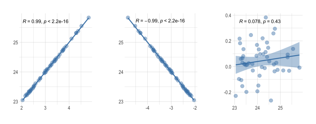
Before reaching a conclusion, it is necessary to conduct a correlation test. We need to test the hypothesis for the significance of the correlation coefficient. The corresponding hypotheses for conducting that statistical test are:

where r is some correlation coefficient. The level of statistical significance is often expressed as a p-value between 0 and 1. The smaller the p-value, the stronger the evidence that we should reject the null hypothesis.

For example, we can interpret p-value of 0.05 as: assuming that the correlation coefficient is zero, we’d obtain the sample effect, or larger, in 5% of studies because of random sample error. For more details explore this link

How to decide which correlation coefficient to use?

Depending on the different characteristics of the data we analyze, we choose the correlation coefficient. So far, we have already mentioned some differences between the correlation coefficients. 

To sum up, there are cases when we recommend the use of certain correlation coefficients.

  • If data is continuous, normally distributed, and does not have outliers we use the Pearson correlation coefficient.
  • Spearman’s rho and Kendall’s tau are nonparametric techniques so we can use them when data is not normally distributed. 
  • Unlike Spearman’s rho, Kendall’s tau is not sensitive, it is more robust to outliers. So, If our data is continuous with outliers we should use Kendall’s Tau. Additionally, we can use it with very small sample sizes.
  • Generally, the disadvantage of rank coefficients is that there is a loss of information when the data is converted to ranks. Also, if the data is normally distributed, it is less powerful than the Pearson correlation coefficient.
  • If one or both variables are ordinal in measurement, we should use a rank coefficients.

Example 3

Let’s examine the connection between CAC and CR a little more. We have already seen, on the first figure, that there is a connection between these variables. When one variable grows, another falls and vice versa. Let’s look at how to find the strength of that connection.

Negative correlation between CAC values and CR.

First, let’s test the normality of this data. The KS (Kolmogorov-Smirnov) test shows that we cannot reject the hypothesis of data normality (at a significance level of 1%), but we do have some visible outliers. So, Pearson’s coefficient is not reliable here. The obtained correlation coefficients are shown in the following table.

Pearson’s

Spearman’s 

Kendall’s 

-0.52

-0.58

-0.39

From interpretation we can conclude that there is a negative correlation between 69.5 % of all possible pairs of data points. The calculation (-0.39 + (1+0.39) / 2 = 0.305)  gives the percentage of positively correlated pairs, which is 26.5 % from which our conclusion follows. 

Example 4

We generated data for this example to visually show the more difference in coefficients. Here we see the true strength of the rank coefficients.

Firstly we compare the Pearson and Spearman correlation coefficients. For all three graphs below, the Spearman coefficient is 1 – there is a monotonic relationship between the variables x and yi (i=1, 2, 3).

As you can see, in the first case, the observed correlation coefficients are equal, the monotonic relationship is linear. In the second case, the monotone connection is a cubic function (y2= x+ c2), so the Pearson coefficient dropped to 0.84. In the latter case, the monotone relation is exponential (y3= exp(x) + c3 ), and the Pearson coefficient is only 0.56.

For cases where the variables do not have a linear trend, but have a trend – the Pearson coefficient is significant. (Because we run a test that compares a linear model and a constant model.)

Representation of decreasing power of rank coefficients in relation to Pearson's correlation coefficient.

Example 5

Next, consider the graph below. We will compare Kendall’s coefficient with Pearson’s: Pearson’s r is 0.7, and Kendall’s tau is  almost 1! This is what Kendall’s tau recognizes in the data, the continuous growth in ranks.

In this case, it shows that there is a positive correlation between 99 % of all possible pairs. On the graph, we see a change in trend after the value x = 40. First, the series moved linearly (with a slope of 0.2), but after some time it began to move with an exponential trend.

The Pearson coefficient recognizes the change in motion, but its value shows a weaker strength. Additionally, in this case, the variables are not normally distributed, so Pearson’s r is not reliable at all.

Another example showing the strength of the Kendall correlation coefficient. (When the data are not linear over the entire observed segment.)

Conclusion

Combinatorial conclusions and basic statistical metrics, such as covariance and standard deviation, allow us to perform many analyses. In fact, the mentioned statistical metrics make correlation theory much more understandable.

For example, the quotient of common variability (covariance) and deviation from the average of the corresponding variables determine the existence of a linear relationship between the data. If the relationship is not linear, we use the rank of correlation coefficients.

According to this link, there is a multitude of different coefficients, most of which are reformulated and upgraded correlation coefficients described in this post. Sometimes the problem we are solving is specific and we need to make modifications to the standard approaches to come to the correct conclusion. 

Additionally, we have shown that there are correlations between many variables in online marketing. This gives us the motivation to detect the trend of a variable using correlation coefficients.

Understand and optimize your performance with Lebesgue

⭐⭐⭐⭐⭐ 

100+ five-star reviews on Shopify App Store

Recommended Posts

No comment yet, add your voice below!


Add a Comment

Your email address will not be published.